What is Deep Learning?
Deep Learning is a branch of Machine Learning which itself is a subset of AI. Deep Learning is inspired from biological neural network and combined with Mathematics it becomes Artificial Neural Network
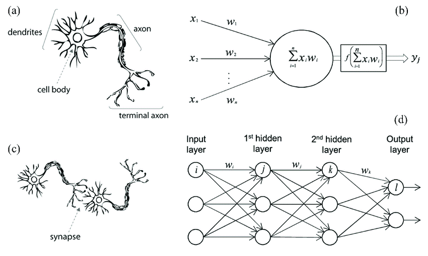
Artificial Neural Network is collection of different layers like input layer, hidden layer & output layer. And these layers are collection of neurons which are also called as perceptron. In a single layer we can have any number of neurons depends on input size or complexity of data.
Starting layer by layer
- Input Layer
- The first layer of artificial neural network is input layer which contains neurons depends on how many features you have in your data
- Hidden Layer
- The second layer is hidden layer and we can have multiple hidden layers depends on complexity of problem. If data is complicated and using a single layer of few neurons is not getting you desired output then you can increase neurons and even hidden layers.
Using Multiple hidden layers makes a deep neural network architecture - Output Layer
- The last layer is output layer which is responsible for doing prediction for your input data.
- Decide whether a neuron should be activated or not.
- It is the non-linear transformation that we do over the input signal.
- Linear function
- Sigmoid or Logistic function
- Tanh Function (Hyperbolic Tangent)
- Softmax Function
- ReLu Functions – Rectified Linear Unit
- Leaky ReLu
- Parametric ReLu
- ELU – Exponential Linear Units
- Swish Function
- GELU – Gaussian Error Linear Unit
- SELU – Scaled Exponential Linear Unit
Now all these layers are connected in a manner that previous layer becomes input for next layer.
The term “Deep” refers to the deep architecture of neural network. Traditional neural network contains only 2 to 3 hidden layers, while deep learning can have any number of layers.

Math Behind Neural Networks
Suppose you have some data which contains 3 features and 1 target

Now our objective is to apply deep learning on this data and find out the predictions for upcoming input values.
First step is to identify number of features we have in our data, here we have 3 features, so we need 3 neurons in our input layer.
Second step is to initialize some random weights that will be multiplied with our input and do sum of all multiplied values. Weights simply represents how strong the connection between the neurons is and how much influence the input will have on neuron’s output. Higher the value of weight higher the influence will be.
Now time for some mathematics

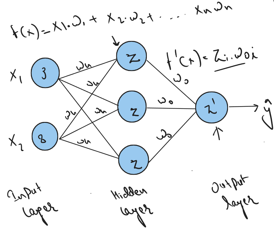
In the above equation we are simply multiplying our input values with some random weights. Weights are initially random because we don’t know that value of weight we should start with.
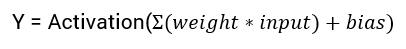
This equation can be re-written as:

Now we introduce one bias term in the above equation. Bias is generally used to move entire activation function (covered later) to the left or right to generate required output values. Bias can also help when we get zero in our equation. In that case bias value will help to not let neuron die.
So the updated equation will look like:

Now we will reach our first hidden layer from input layer. Here the role of hidden layer is to apply some activation function to simply activate the neuron available in hidden layer.
What are Activation Functions?
Can we do without an activation function?
A linear equation is simple to solve but is limited in its capacity to solve complex problems. A neural network without an activation function is essentially just a linear regression model.
The activation function does the non-linear transformation to the input making it capable to learn and perform more complex tasks.
We would want our neural networks to work on complicated tasks like language translations and image classifications.
Now our equation will become:
List of few popular activation functions
Suppose if we use sigmoid activation function then equation will look like:
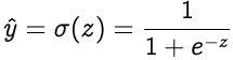
Where σ denotes the sigmoid activation function.
Now from hidden layer we will move towards the output layer and output layer will also apply some activation function on input coming from the hidden layer.
This whole process is known as feedforward
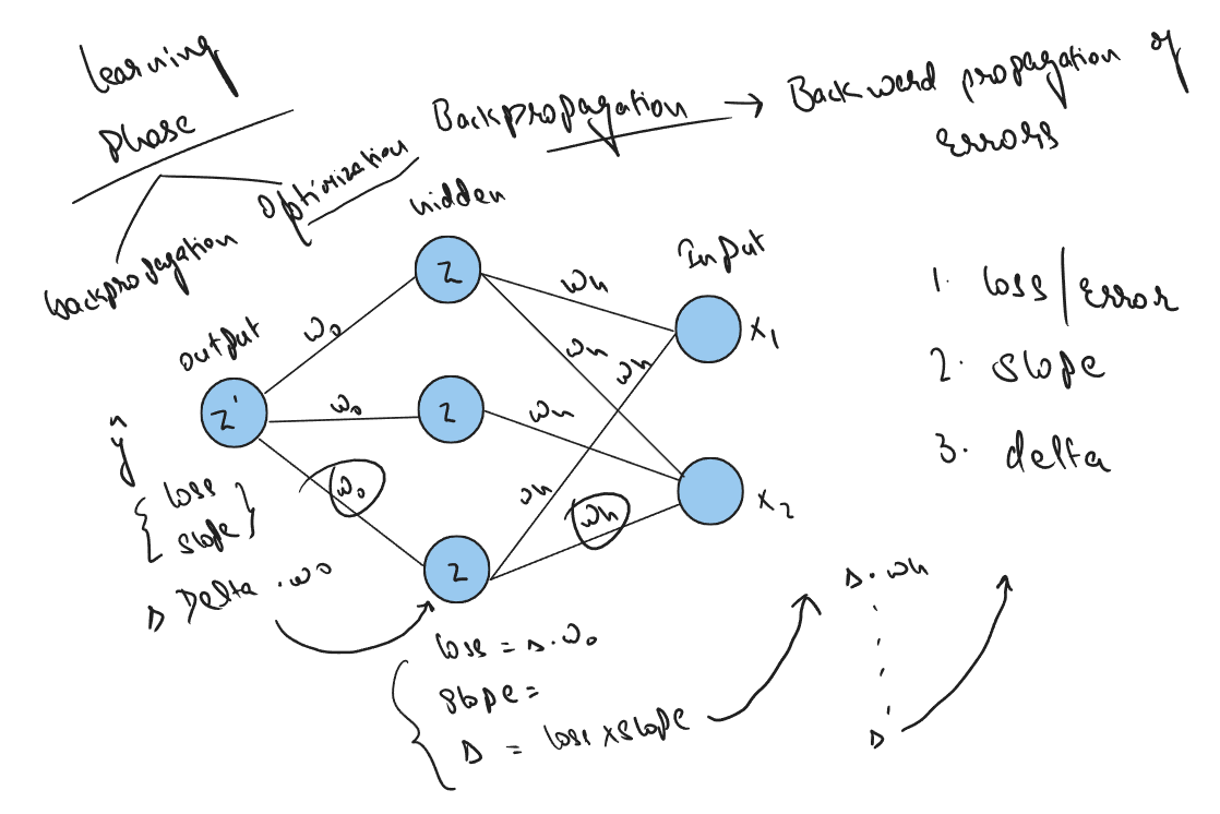
Now comes the learning part of our deep learning algorithm that is Backpropagation, where we optimize the model by updating the weights on each layer.
In backpropagation we compute the gradient of loss function with respect to weights.
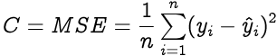
So the first step is to find out error on output layer by simply calculating the difference between actual (yᵢ) and predicted value ( ŷᵢ ).

Loss function is calculated for the entire training dataset and their average is called the Cost function C.
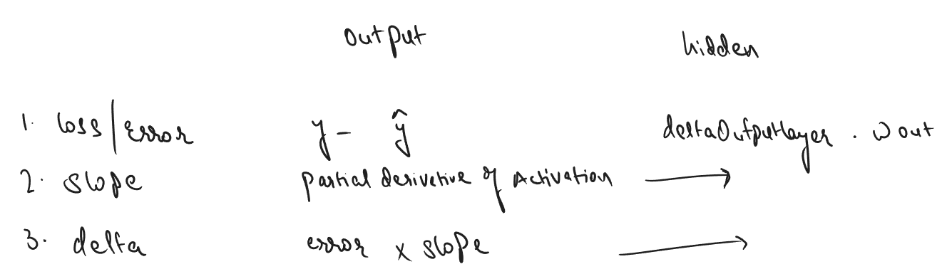
In backward propagation we need to find out 3 things on each layer
- Loss
- Slope
- Delta
For Ouput layer
loss is : actual - predicted value that we have already talked about,
slope is simply the derivative of activation that we used,
delta is error times the slope : delta = error x slope
For Hidden layer
loss is : dot product of previous layer's delta and weights at the layer,
slope is simply the derivative of activation that we used,
delta is error times the slope : delta = error x slope
After calculating the backpropagation part we need to optimize our weights and bias until model convergence

That’s it and after the convergence of model we can start doing prediction using our updated wights and bias value.
You can find out the python implementation of ANN from Scratch here
Hope you find this article useful and understood the concept of deep learning mathematically and theoretically as well.