What we are gonna cover?
- What is an optimizer?
- Types of Optmizers
-
Gradient Descent
- Batch Gradient Descent
- Stochastic Gradient Descent
- Mini Batch Gradient Descent
- Momentum
- NAG - Nestrov Accelarated Gradient
- AdaGrad - Adaptive Gradient
- AdaDelta
- RMSProp
- Adam - Adaptive Moment Estimation
- AdaMax
- Nadam
- AMSGrad
The learning phase of a deep learning model is divided in 2 parts
- Calculating Loss
- Optimization of weights and bias
We have already covered the loss functions in deep learning, now let's talk about Optimizers...
What is an Optimizer?
So far we know about how loss functions tells us about how well our model is fitted on current dataset. Now when we get to realize that our model is performing poor at the current instance so we need to minimize the loss and maximize the accuracy. That process is known as optimization.
Optimizers are methods or algorithms used to change the attributes of neural network such as weights and learning rate to reduce the loss.
After calculation of loss we need to optimize our weights and bias in the same iteration.
How do Optimizers work?
To understand working of optimizers just think of a situation...
You are somewhere on top of a mountain with a blindfold on. Now you have to get down from the mountain to reach your home safely.
What will be your approach...???
You have to take one step at a time and if you are going down then it makes you making some progress but if you are going up then you are going in wrong direction.
So you will start doing hit and trial and take steps that will lead you downwards.
Similarly our optimization techniques works. Initially we don't know the weights so we start randomly but with some trial and error based on loss function we can end up getting our loss downwards.
Optimization techniques are responsible for reduing the loss and provide most accurate results possible.
There are various optimization techniques, we'll learn about different types of optimers and how do they work to minimize loss.
Gradient Descent
Gradient Descent is one of the popular techniques to perform optimization. It's based on a convex function and yweaks its parameters iteratively to minimize a given function to its local minimum.
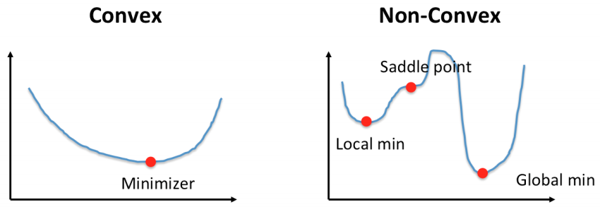
Gradient Descent is an optimization algorithm for finding a local minimum of a differentiable function.
We start by defining initial parameter's values and from there gradient descent uses calculus to iteratively adjust the values so they minimize the given cost-function.
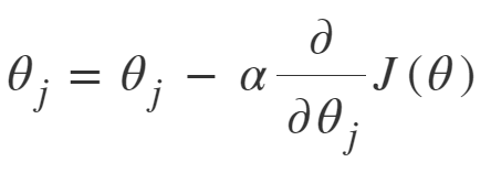
The above equation computes the gradient of the cost function J(θ) w.r.t. to the parameters/weights θ for the entire training dataset:
"A gradient measures how much the output of a function changes if you change the inputs a little bit." — Lex Fridman (MIT)
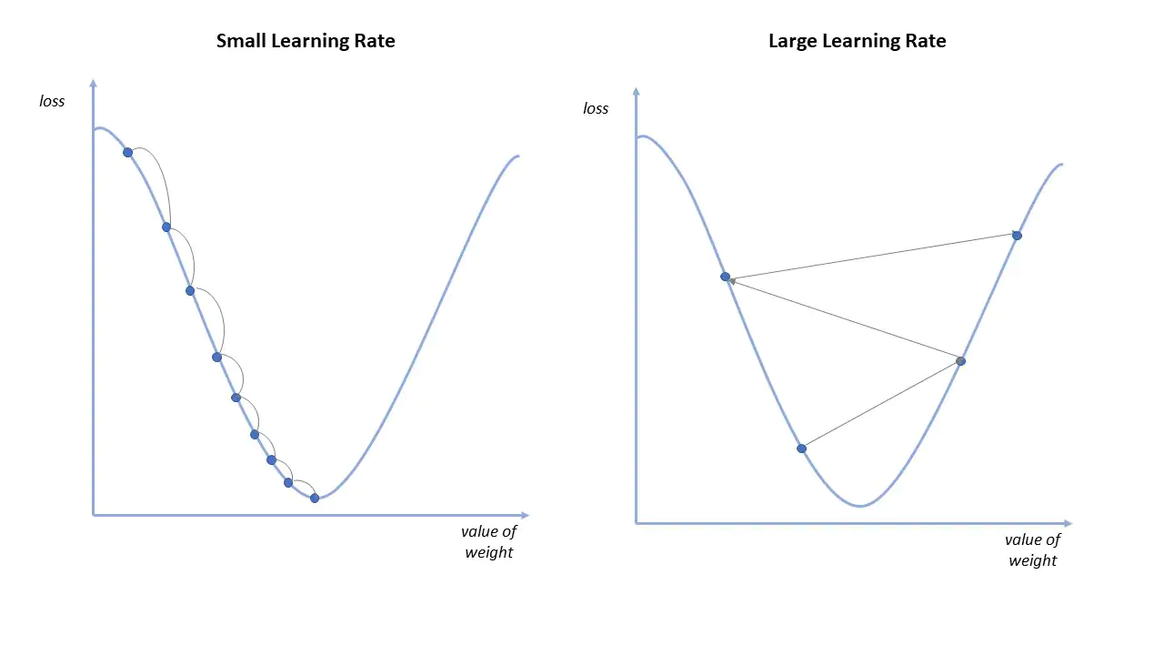
Importance of Learning Rate
Learning rate determines how big the steps are gradient descent takes into the direction of local minimum. That will tells us about how fast or slow we will move towards the optimal weights.
When we initialize learning rate we set an apporpriate value which is neither too low nor too high.
Advantages of Gradient Descent
- Easy Computation
- Easy to implement
- Easy to understand
Disadvantages of Gradient Descent
- May trap at local minima
- Weights are changed after calculation the gradient on whole dataset, so if dataset is too large then it may take years to converge to the minima
- Requires large memory to calculate gradient for whole dataset
3 Types of Gradient Descent
- Batch Gradient Descent
- Stochastic Gradient Descent
- Mini Batch Gradient Descent
Batch Gradient Descent
In batch gradient descent we uses the entire dataset to calculate gradient of the cost function for each epoch.
That's why the convergence is slow in batch gradient descent.
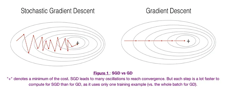
SGD - Stochastic Gradient Descent
SGD algorithm is an extension of the Gradient Descent and it overcomes disadvantages of gradient descent algorithm.
SGD derivative is computed taking one observation at a time. So if dataset contains 100 observations then it updates model weigts and bias 100 times in 1 epoch.
SGD performs parameter updation for each training example x(i) and label y(i):

where {x(i), y(i)} are the training examples
Stochastic Gradient Descent vs Batch Gradient Descent
Advantages of SGD
- Memory requirement is less compared to Gradient Descent algorithm.
Disadvantages of SGD
- May stuck at local minima
- Time taken by 1 epoch is large compared to Gradient Descent
MBGD - Mini Batch Gradient Descent
MBGD is combination of both batch and stochastic gradient descent. It divides the training data into small batch size and performs updates on each of the batch.
So here only subset of dataset is used for calculating the loss function.
Mini Batch is widely used and converges faster because it requires less cycles in one iteration.

Advantages of Mini Batch Gradient Descent
- Less time taken to converge the model
- Requires medium amount of memory
- Frequently updates the model parameters and also has less variance.
Disadvantages of Mini Batch Gradient Descent
- If the learning rate is too small then convergence rate will be slow.
- It doesn't guarantee good convergence
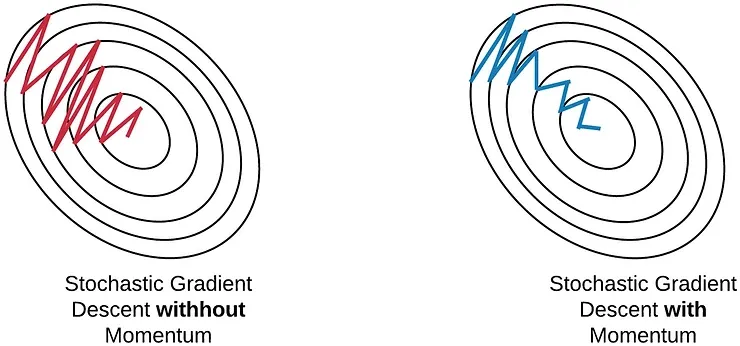
Momentum
Momentum was introduced for reducing high variance in SGD. Instead of depending only on current gradient to update weight, gradient descent with momentum replaces the current gradient with V (which stands for velocity), the exponential moving average of current and past gradients.
Momentum simulates the inertia of an object when it is moving, the direction of the previous update is retained to a certain extent during the update, while the current update gradient is used to fine-tune the final update direction.
One more hyperparameter is used in this method known as momentum symbolized by ‘γ’.
V(t)=γV(t−1)+α.∇J(θ)
Now, the weights are updated by θ=θ−V(t).
The momentum term γ is usually set to 0.9 or a similar value.
Momentum at time ‘t’ is computed using all previous updates giving more weightage to recent updates compared to the previous update. This leads to speed up the convergence.
Essentially, when using momentum, we push a ball down a hill. The ball accumulates momentum as it rolls downhill, becoming faster and faster on the way (until it reaches its terminal velocity if there is air resistance, i.e. γ < 1). The same thing happens to our parameter updates: The momentum term increases for dimensions whose gradients point in the same directions and reduces updates for dimensions whose gradients change directions. As a result, we gain faster convergence and reduced oscillation.
Advantages
- Converges faster than SGD
- All advantages of SGD
- Reduces the oscillations and high variance of the parameters
Disadvantage
- One more extra variable is introduced that we need to compute for each update
NAG - Nesterov Accelerated Gradient
Momentum may be a good method but if the momentum is too high the algorithm may miss the local minima and may continue to rise up.
The approach followed here was that the parameters update would be made with the history element first and then only the derivative is calculated which can move it in the forward or backward direction. This is called the look-ahead approach, and it makes more sense because if the curve reaches near to the minima, then the derivative can make it move slowly so that there are fewer oscillations and therefore saving more time.
We know we’ll be using γ.V(t−1) for modifying the weights so, θ−γV(t−1) approximately tells us the future location. Now, we’ll calculate the cost based on this future parameter rather than the current one.

and then update the parameters using θ = θ − V(t)
Both NAG and SGD with momentum algorithms work equally well and share the same advantages and disadvantages.
AdaGrad - Adaptive Gradient Descent
AdaGrad is little bit different from other gradient descent algorithms. In all the previously discussed algorithms learning rate was constant. So here the key idea is to have an adaptive learning for each of the weights.
It uses different learning rate for each iteration. The more the parameters get change, the more minor the learning rate changes.
Lot of times we have sparse as well as dense dataset, but we keep our learning rate constant for all the iterations.
AdaGrad uses the formula to update the weights:

Here the alpha(t) denotes the different learning rates at each iteration, n is a constant, and E is a small positive to avoid division by 0.
Advantages
- Learning rate changes adaptively, no human intervention is required
- One of the best algorithm to train on sparse data
Disadvantage
- Learning rate is always decreasing which leads to slow convergence
- Due to small learning rate model eventually becomes unable to train properly and couldn't acquire the required knowledge and hence accuracy of the model is compromised
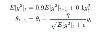
AdaDelta
AdaDelta is an extension of AdaGrad. In AdaGrad learning rate became too small that it might decay or after some time it approaches zero.
AdaDelta was introduced to get rid of learning rate decaying problem.
To deal with these problems, AdaDelta uses two state variables to store the leaky average of the second moment gradient and a leaky average of the second moment of change of parameters in the model.
In simple terms, AdaDelta adapts learning rate based on a moving window of gradient update, instead of accumulating all past gradients.
Here exponentially moving average is used rather than sum of all the gradients.
E[g²](t)=γ.E[g²](t−1)+(1−γ).g²(t)
We set γ to a similar value as the momentum term, around 0.9.

Advantages
- Learning rate doesn't decay
Disadvantages
- Computationally Expensive
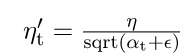
RMSProp - Root Mean Square Propagation
RMSProp is one of the version of AdaGrad. It is actually the improvement of AdaGrad Optimizer.
Here the learning rate is an exponential average of the gradients instead of the cumulative sum of squared gradients.
RMS-Prop basically combines momentum with AdaGrad.
RMSprop as well divides the learning rate by an exponentially decaying average of squared gradients. Hinton suggests γ be set to 0.9, while a good default value for the learning rate η is 0.001.
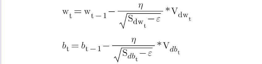
Adam - Adaptive Moment Estimation
One of the most popular optimization techniques is Adam. It computes adaptive learning rate for each parameter. It is actually the combination of RMSProp and SGD with Momentum.
It stores both the decaying average of the past gradients , similar to momentum and also the decaying average of the past squared gradients , similar to RMS-Prop and Adadelta. Thus, it combines the advantages of both the methods.
It also introduces two new hyper-parameters beta1 and beta2 which are usually kept around 0.9 and 0.99 but you can change them according to your use case.
Advantages
- Computationally Efficient
- Memory Efficient
Conclusion
Adam is one of the best optimizer and if you have sparse data then use optimizers with dynamic learning rate.
So far we have covered all the popular optimization techniques but still there are few more optimization techniques that you can try.
Hope you enjoyed learning from this blog.